Free online course Microsoft Excel 2010 Part 1

[forums]

Everyone in the corporate life has made use of Microsoft Excel to a certain degree. And almost everyone know that colleague with his ‘lease car file’. Through a series of three blogs that go up in difficulty each time I will discuss several Excel functions and formulas. After this you can also create your own useful and time saving Excel files with ease.

Before we start the Excel course

Before we start it is useful to ensure that we have both set the same language in Microsoft Excel 2010. This is because this has effect on the names of the functions and therefore prevents a lot of confusion of tongues and searching.

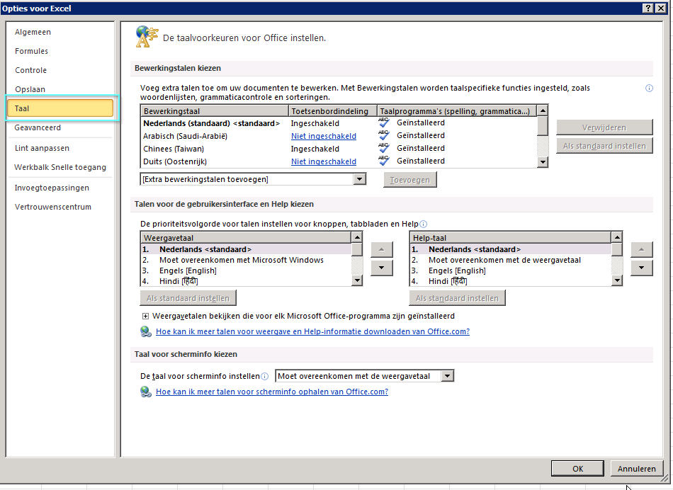
In Microsoft Excel 2010 you change the language by clicking on ‘File’ and subsequently on ‘Options’. After this the screen ‘Options for Excel’ appears.

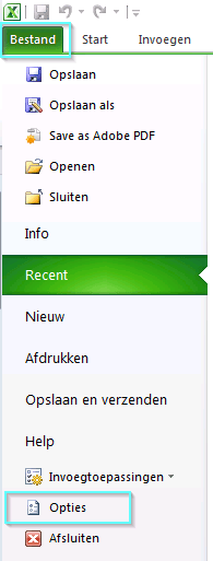
Click here on ‘Language’ and change the language to ‘Dutch’.

Now that this is arranged we can begin.

What will we learn during this Excel course?

To make something recognizable I will cover the earlier mentioned Excel functions and formulas by means of a case.

During this blog we are the accountant of ‘Jansen Gardening.’, a starting wholesale that trades with products of the brands Gerdana, Hurvasqa, Forrest, and Fern. Business is booming at Jansen Gardening and more and more is being sold. As is the case for many starting companies the sales invoices of the company are still created with Microsoft Excel and subsequently checked into the accounting system. There is of course nothing wrong with that in itself, but not more and more is being sold it takes up a lot of time to manually calculate and enter all fields. To quicken this process and automate it we will extend the Excel file.

In this first blog I will cover the following topics:

• How do I handle this?;
• How do I create the layout of the file?;
• How do I create simple mathematical formulas (minus/plus,multiplication, etc.)?

In the second blog of this series I will cover several functions for more advances users, such as:

• How do I use the sum-formula ( =sum() );
• How do I use the if-formula? ( =if() );
• How do I use the search vertically formula? ( =vert.search() );
• How do I secure my Excel file?

In the third blog I will cover the following functions for further advanced users:

• How do I make use of buttons?;
• How do I make drop-down menus?;
• How do I make macros?

During this blog I will make use of Microsoft Excel 2010. I have chosen for this because for companies this is the most user version. Older versions of Excel have virtually all functions of Excel, but versions before Microsoft Office 2007 do have a different layout.

As indicated above I will first start to explain how I handle the creation of Excel files with many and often large formulas.

How do I go about the creation of an Excel sheet?

You will see that the more experience you acquire with Microsoft Excel, the more extended the files and formulas will become. It may sound a little surreal now, but it might happen that you will get formulas that do not fit in the formula bar at once.

To retain the overview and find possible non-operative formulas, I think it is required to use a structured approach.

For the creation of a new Excel file I use roughly the following steps:

1. Create or open the base file. This is a version with just the layout of the file.
2. Fill in test data. Fill in all input fields like you would have normally done manually. This is all just text. This way you can test later on whether your formulas work.

Now you really already have a usable file. What we will now do is use the functions of Microsoft Excel to ‘smarten’ the file.

3. Start by adding some simple formulas. Think of the usual mathematical formulas like A/B=C.
4. Add the more complex formulas. You can for example think of formulas that keep cells empty based on certain conditions,
5. Add advances functions. Think for example of buttons that immediately print the file. Now it is clear how to create an extended Excel file we will execute step one in the following paragraph.

How do I change the layout in Excel?

Every file really looks differently. An invoice will of course look differently than a payslip. But even invoices nearly always differ from each other.

Before we start to randomly place formulas it is useful to organize the layout of the file. Otherwise you will create formulas that you need to move later on. First we will look at where to find the different functions in Excel to create the layout. Then we will cover how to use these functions to create the layout. To supply you with an idea of what we are working towards, and as useful source for images and icons you can download an Excel file with the final result of this blog by clicking on the image below.

Functions for layout

You will probably not be creating work of art in Microsoft Excel with the options I describe below (although it is ), but almost anything is possible within reason. Most options for the layout of the file can be found under the tabs ‘start’ and ‘insert’

Under the tab ‘start’

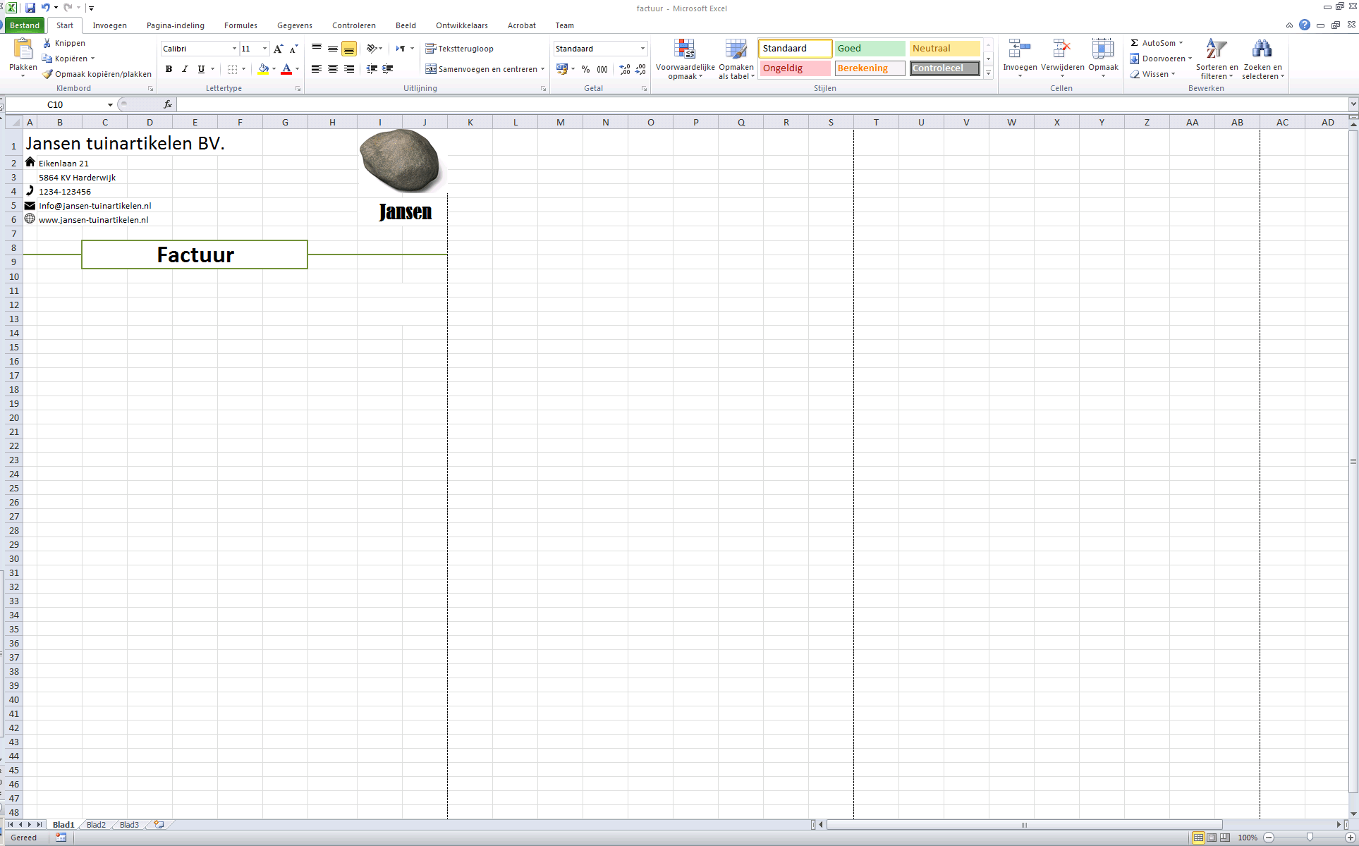
Most functions can be found under this tab that are needed for the layout of your Excel file. Here you will find the possibility to cut, copy, and paste, functions for the layout of the text, and functions for the layout of grid lines and cells.

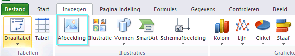
Under the tab ‘insert’

The functions under the tab insert that you will primarily use are those to add images or shapes. For the insertion of images you can of course also just use the windows shortcuts ctrl-c (for copy) followed by ctrl-v (for paste).

Creating the lay-out

Before we begin I should note that the creation of the layout is a bit of trial-and-error work. It is possible that everything is as it is supposed to be up in the file, and that you then discover that further down you do really need an extra column.

That said, we can begin with the creation of the invoice layout. First we will look at the placement and adjustment of text, and the placement of images. Then we will cover the adjustment of cells and borders.

Text placement and adjustment and inserting images

The first thing to be done now is to learn how to insert text and give it layout in Excel. Subsequently we will cover how to insert images.
In the upper left we would like all contact data of our own company. For the layout of this we have the following wishes:

1. The company name should be bigger than the standard and it should be printed in bold,
2. the telephone number, E-mail address, and the address of the website are to be smaller than the standard,
3. Images should be used instead of the words ‘Phone number’, ’E-mail’, ’Address’, and ‘Website’ to indicate which information is concerned,
4. The logo should be placed in the upper right corner.

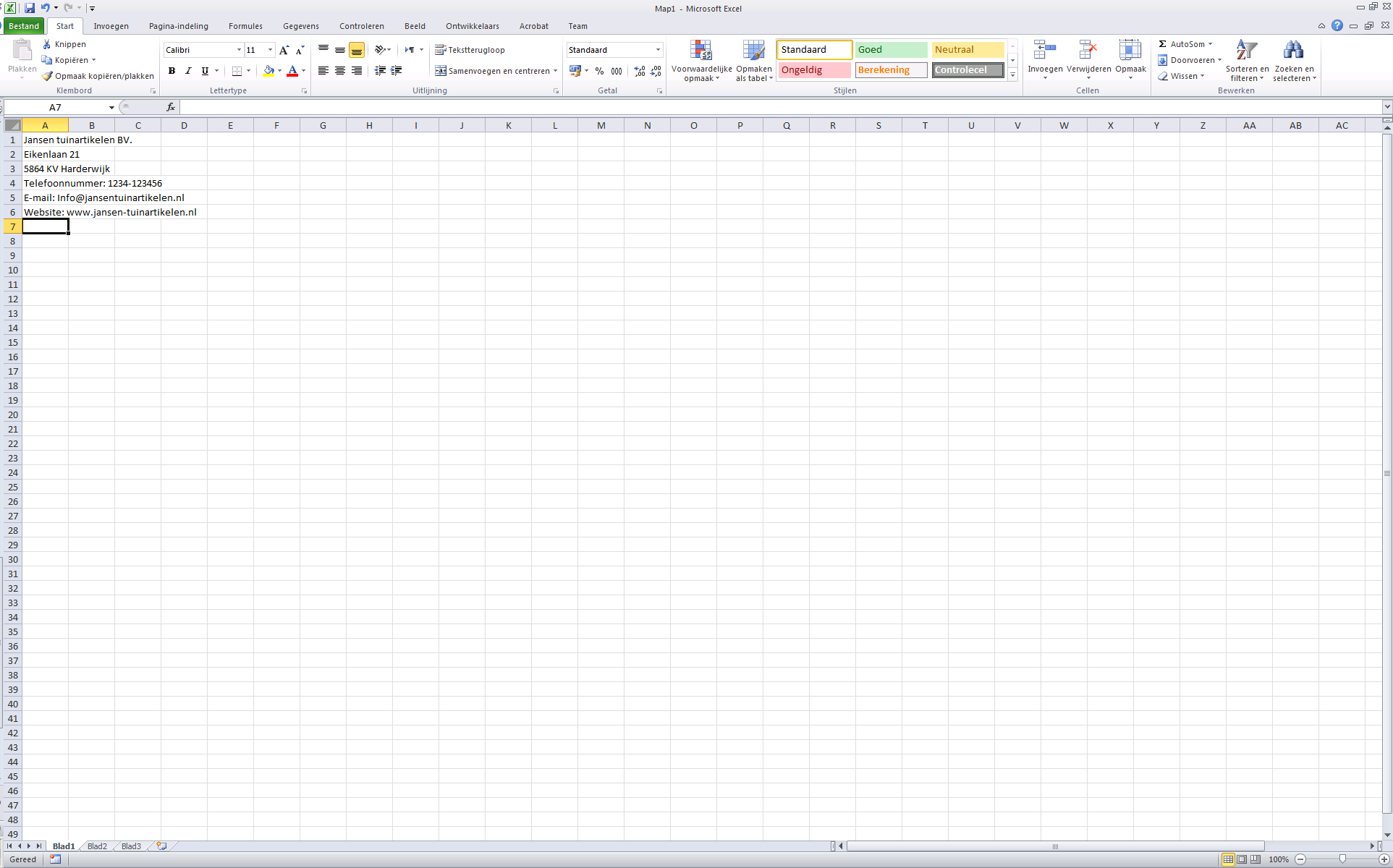
First we start with the typing of the data in separate cells. This is to be done as follows:

1. Click on the cell in which you would want to have the text,
2. Type the text,
3. Go to the following cell. This can be done by:
   1. Clicking on the cell;
   2. Using the enter key.

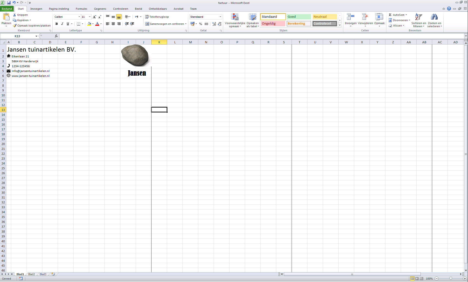
Now copy the text of the image below.

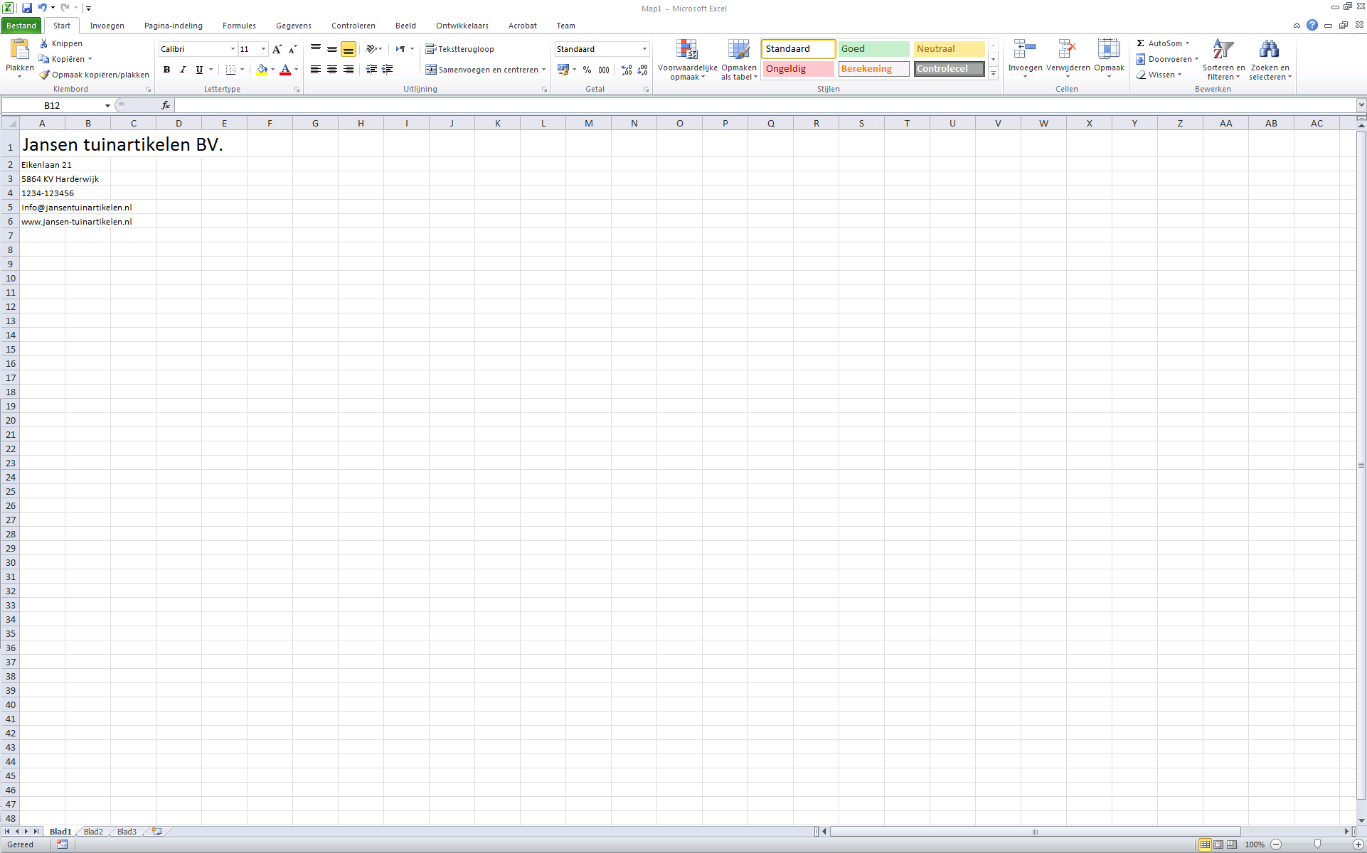
Now we have filled the cells with text we will proceed to determine the layout of this text. We start with wish number one, making the text larger and in bold. This is to be done as follows:

1. Click on the cell that you wish to adjust,
2. Now change the layout of the text by using the functions ‘font size’ and ‘bold’.

These options can be found in the menu Start as depicted in the image below.

Now make sure that your Excel file looks exactly like the image below. The company name should be one size larger than standard, and the other data one size smaller.

Now we have covered the first topic, it is time to work on our second wish. Inserting images to indicate which information is concerned in the invoice header.
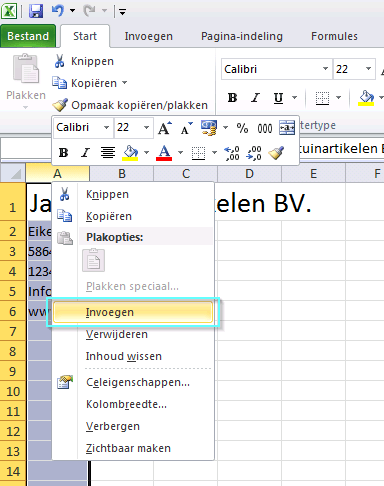
As you might have noticed already, there is no space left anymore before the text. We can solve this by adding an extra column. This is to be done as follows:

1. Now right click on column ‘A’,
2. Now click on the option ‘Insert’.

Now that you have added a column there is enough space to place the images. This can be done by copying the images from the source location and then paste them in the file. This can be done in two ways. That is by using the function for inserting images, or the Windows shortcuts for copying and pasting.

Adding images using the function inserting images can be done as follows:

1. Select the cell in which you would want to have the image,
2. Now go to the tab ‘Insert’ and select ‘Images’ there,
3. Now search through the usual Windows screen for the folder with the image in it
4. Select the correct image and click on ‘Insert’.

Adding images using the Windows shortcuts is done as follows:

1. Search for an image you wish to use,
2. Select the image by clicking on it,
3. Now use the button combination ‘CTRL’ and ‘c’ to copy the image,
4. Click on the location in the Excel file where you would like to position the image,
5. Now use the button combination ‘CTRL’ and ‘v’ to paste the image.

The first method is especially easy to use whenever the image is located somewhere in a folder on the computer. The second option is best used whenever the image is from a different file or from the internet.

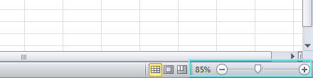
Of course everything should be aligned neatly. This can be done by making use of the cell next to it or, in this case, the margin. This can best be seen by zooming in on the sheet. In Microsoft Excel you can zoom by use of:

1. The scroll button on your mouse,
2. The zoom buttons of Excel.

The last method is shown below.

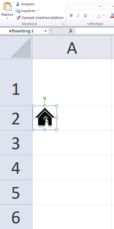
Now you are zoomed in you can align the images. To make this a little easier it is best to choose icon from one type of series. This way the distance between the edge of the image and the image itself should usually be equal. Of course it also looks a lot neater when everything is done in the same style.

Aligning the image is done as follows:

1. Select the image. A line around the image will appear,
2. Slide this line precisely against the border of the bordering cell. In this case this is the margin line.

You might have noticed already that when we entered a new column the company name also moved. We still have to put that neatly back in place. This is done by cutting and pasting the cell with the company name in it. This is to be done as follows:

1. Select the cell in which the text is in now,
2. Now cut the cell by using the shortcut ‘CTRL’ and ‘x’.
3. Select the cell where the text is to be copies towards. In this case this is cell A1.

Now we are done with wish 2. All that remains is the placement of the logo of Jansen Gardening in the upper right corner of the file. Before you can do this you do need to know where this upper right corner is. You can learn this by displaying the print range of the file in the Excel file itself. This is to be done as follows:

1. Go to ‘File’,
2. Now click on ‘Print’,
3. Now go back to the tab ‘Start’.

You can see that multiple dotted lines have appeared. These are the print ranges. These print ranges indicate what fits onto 1 page should you print these. Since we want to have the invoice on the first page, we will use the print range between the left margin and the first subsequent dotted line, and the upper margin and the first subsequent dotted line.

Now that we know this we can align the logo against the right side of our print range. First paste the logo into the Excel file and then align it against the right side. This can be done the same away as you have done with the icons earlier.

Adjusting the borders and cells

Now that we know how to adjust the text and place image, we need to learn how to format the lines and cells. This will really allow you to make the invoice properly clear.

We will not place a line to indicate where the header and where the body of the invoice is. Placing a line is done as follows:

1. Go to the tab ‘Start’,
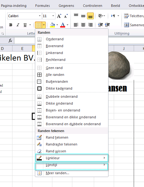
2. Click here on the option ‘border’. Here there are various options for the formats of the cell lines,
3. Here, for ‘line color’, you can pick the color you want the lines to have, green in this case,
4. For ‘line style’ you can pick the type of line you would want to have. In this case we choose the bold uninterrupted line,
5. The cursor of your mouse now changes to a little pencil. Now select the lines you wish to provide this format to.

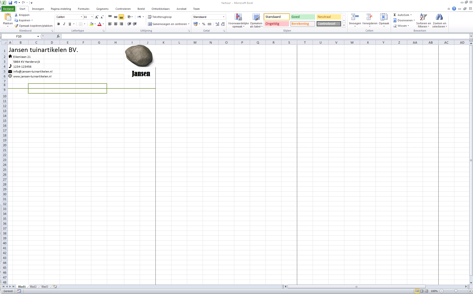
Now add lines using the example below.

Before you can go underway with the rest of the layout there are still three functions I will cover. The first of these is the function ‘Merge and center’. The second is the alignment of text in cells. Then I will cover how to adjust the format of a cell for currencies.

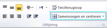
The function Merge and Center can be found in the menu Start.

If you look at the Excel file you can see that space has been left in the layout in the shape of a rectangle. Here we will neatly place the word ‘Invoice’ centered. However, as you can see from the green line the block consists of two layers of cells.

By using the function ‘Merge and center’ you can merge multiple cells into one big cell without affecting the other cells in the rows and columns. In addition, it automatically centers the content that you type in the new cell. This function is to be used as follows:

1. Select the cells you wish to merge,
2. Click on the button ‘Merge and center’,
3. Type the text desired by you in your new cell.

However, what if you do not want to have the text centered in the cell, but aligned in a different way? This alignment can be easily adjusted by making use of the buttons below under the tab ‘Start’.

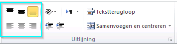
The buttons above will provide you with the possibility to align the text both horizontally as well as vertically. Using the upper three buttons, you can align your text respectively above, in the middle and below in the cell. The bottom three buttons are used for aligning the text left, centered and right.

Now make sure that your Excel file looks the same as the image below.

Since we are busy creating an invoice there are various fields that will always contain a currency number. However, formulas do not work in Excel when text and numbers are used mixed together in a cell. After all, the sum ‘€+€’ does not exist. To provide the contents of a cell with which you will be calculating later on with a currency layout already use the button ‘Financial number format’ in the tab ‘Start’.

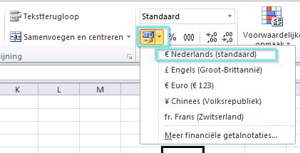
To provide a currency format layout to a cell you do the following:

1. First select the cell,
2. Now click on the button ‘Financial number format’,
3. Now select ‘€ Dutch (standard)’.

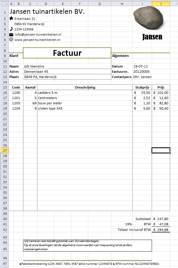
You now know all functions needed to further complete the layout of the file itself. Now try to use the just learned functions to copy the example below. For the subsequent steps it is vital that you copy the example exactly.

How do I make simple mathematical formulas using Microsoft Excel?

The file you have just made is really already usable. And similar files are also just used for some (mostly smaller) companies for billing. But you might have noticed already that, even now the invoice itself is already finished, there is still a lot of time needed for entering and calculation of the numbers. A few small adjustments in the file can save you a lot of time here. We will now look at how a few simple mathematical calculations in the Excel file can simplify the filling out of the invoice.

You can basically look at Microsoft Excel as being an extended calculator. All mathematical calculations that you might do with the calculator can also be done with Microsoft Excel. This is called a ‘formula’ in Excel. Sometimes there are even pre-programmed functions for certain calculations. I will cover some of these functions in one of the next blogs. Now we shall see how Excel deals with formulas. Next we will look at formula creation in Excel.

How does Excel think?

As said we will first look at the creation of simple calculations using Microsoft Excel. Excel normally always considers the text that is entered as ‘flat text’. This means that it will just consider a sum as ‘2+2=’ as text and will not do anything with it.

To clarify to Excel that the text in a cell is a calculation you need to use the ‘=’ character. In your mind you can replace the ‘=’ character for ‘The value that his cell displays is the result of’. So if I want to have a cell that displays the result of the sum ‘2+2’ then I need to type ‘=2+2’. The value that the cell then displays is ‘4’.

This trick Excel can also do when you use it to make a calculation on the basis of the values in two other cells. Furthermore, he will automatically recalculate the result whenever you adjust the values in the other cells (useful!!!).

Perhaps you saw this one coming, but we are going to use this function to take on a lot of calculation work for us in the just made Excel file.

How do I create a formula using Excel?

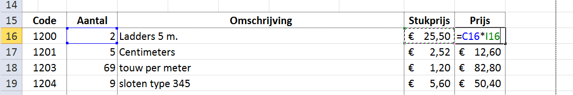
Now that we know how Excel ‘thinks’ we can let him take over some our work. In the example the value that is displayed in the column ‘Price’ (cells J16 through J38) is the result of the multiplication of the values in the column ‘Number’ (C16 through C38) with those in the column ‘Unit price’ (I16 through I38). You might have just calculated this yourself or possibly using a calculator. Now we will let Excel calculate this.

A calculation in Excel is done like this:

1. First you click in the cell in which you wish to display the result of the total. In this case cell J16,
2. Now you type the ‘=’ symbol,
3. Now that Excel knows that you want it to calculate something you select the first variable in cell C16 followed by the ‘multiply’ character (in Excel you use the ‘*’ for this purpose),
4. Then you select the second variable and press the ‘enter’ button.

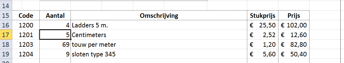
If all is well, you will no see the same number as you calculated manually earlier. This way you can monitor the formula.

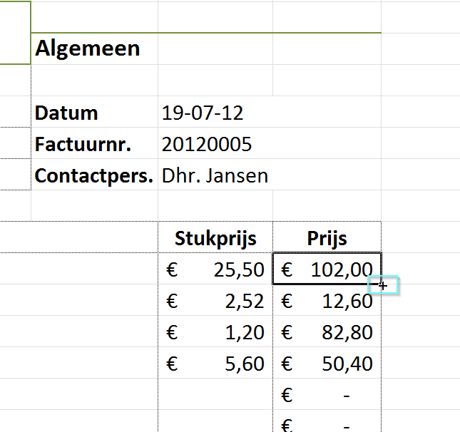
However, when you change the values in the variable cells, for example the number of two to four, then Excel recalculates the result.

Now that we have discussed this trick you can enter the other calculations yourself in Excel. “Sure”, is what you are thinking now, “now I have to enter the same formula over 20 times under the column ‘Price’. Can that not be done with more ease?”. Yes, of course, that is possible. Excel knows that the formula consists of two variable cells. If you ‘extend’ this formula downward it will automatically fit the two variables into the formula towards the cells below it. In other words, formula ‘cell J16 =C16I16’ will automatically change into ‘Cell J17 =C17I17’.

This ‘extension’ of a formula can be done by first clicking on the cell with the formula. Then you grab the small thickening in the right corner below and draw it downwards with you.

Should you accidentally adjust the layout by the dragging of this cell, then you can always edit these again with the functions intended for that purpose.

Please note that Excel can add an at-sign (“@”) automatically to the front of an Excel formula to indicate it operate solely on a single cell as opposed to matrix formulas. For more information: see @ (at-sign) appears in Excel formulas, sometimes breaking formulas.